Support Vector Machine algorithm with mathematical derivation and numpy implementation

Machine learning(ML) is an application of artificial intelligence (AI) ,where the system learns automatically and improves the performance from experience without being explicitly programmed.

Regression and Classification are types of ML algorithms.

Classification is a type of supervised learning. It predicts the class of the given data point.

Support Vector Machine (SVM) Classifier:

SVM is a supervised Machine Learning Algorithm used predominantly for Non-linear Classification type of data modelling. It is used in a variety of applications such as face detection, handwriting recognition and classification of emails.

It employs the concept of using a hyper-plane to separate the data sets into classes. If there are ‘n’ features,’n-1’ dimension hyper-plane will be used i.e. for a 2-D space hyper-plane will be a line ,in case of a 3-D space hyper-plane will be a plane and so on. Support Vectors are the co-ordinates of individual observation.

Hyper-plane selection:

Following are the conditions based on which the right hyper-plane will be selected:

1. If there are a number of hyper-planes, the one which well-segregates the feature is selected.

2. Margin:

Distance of the hyper-plane from the nearest data point is called a Margin. Maximizing the margin helps to find the right hyper-plane. If we select hyper-plane with low-margin then there will be high chance of misclassification, so selecting the hyper-plane with high distance will increase the robustness.

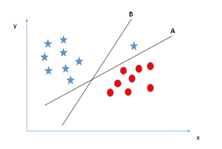
3. Prior to classifying based on the Margin, SVM selects the hyper-plane which classifies the data points accurately.In this case the right hyper-plane is A though hyper-plane B has high margin.

4. SVM has a feature to ignore Outliers and choose the hyper-plane with maximum margin.

Soft Margin is a technique used primarily with Non-linear data to tolerate the one or few misclassified points.

Applying soft margin, tries to balance the trade-off between finding a line that maximizes the margin and minimizes the misclassification.

The amount of tolerance (soft) is an important user-defined parameter for SVM. In Scikit learn,it is represented as the penalty term ’C’. Higher the value of C , SVM gets more penalty when it makes misclassification , narrowing down the margin by considering only a few support vectors for decision-making. Hyper-parameter tuning with various values can be done (will be discussed later in the chapter) to find the best value of C for the model.

5. Hyper-plane for Non-linear data is selected by introducing a new feature Z, which is calculated as follows,

where N is the number of chosen features for the analysis.

Z will always have a positive value as it is the squared sum of the features.
Data points closer to origin will have a smaller value of Z whereas value of Z will be higher for data points away from the origin.

SVM uses the Kernel Trick which takes the existing features, applies transformation and returns new features which are then used for finding the decision boundary .Kernel parameter selection is very helpful in Non-linear classification problems where complex data transformation techniques are used to convert the non-separable data to separable data based on the input features. Multiple choice of kernels like ‘linear’,’polynomial’,Radial Basis function(rbf) are available.Polynomial and rbf are best suited for Non-linear data.

Gamma is an important parameter in rbf, which controls the influence of the new features on the decision boundary.Higher the value of gamma will create impact on the adjacent data points.Lower the better.we can choose the Kernel and gamma values best fitting our model using the hyper-parameter tuning(discussed later in the section).

SVM Mathematical Derivation:

Hyper-plane equation for Linear data:

In case of 2-D space, the hyper-plane to separate the classes will be a line.

Considering the line equation,

y=ax+b

mx+c-y=0

Let us consider X=x,y and W as (a,-1),then the above equation becomes,

W.X+c=0

Most of the real-time scenarios will have non-linearly separable data. In this case a new feature will be introduced (discussed earlier in point 5 of hyper-plane selection) to classify the data points.

Any hyper-plane can be written as the set of points x satisfying w⋅x+b=0 --(1)

Compute Margin of the hyper-plane:

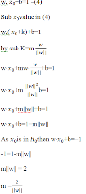
We have found the formula to calculate the margin. Minimum the norm(||w||) maximum will be the Margin (m).

Let’s explain margin calculation with an example:

Orthogonal projection of a vector and Dot product of the vectors are the concepts used to compute the distance of a data point from the hyper-plane.

To find distance between the vector w(2,1) which is normal to the hyper-plane and a(3,4),we consider a projection vector P from w:

SVM Implementation:

Hyper-Parameter Tuning:

There are number of parameters in SVC which help to improve the performance of the data model.

Kernel, Gamma and C are the most important of them.

Cross validation is a method for evaluating models. To find the optimal hyper-parameters, we take a set of candidate hyper parameters, train models for all of these and compare their fitness via cross validation. Finally we select the hyper-parameters that gave the best CV score.

To choose the best values for these parameters the following approaches are used.

GridsearchCV is commonly used as an approach to hyper-parameter tuning that will methodically build and evaluate a model for each combination of algorithm parameters specified in a grid.(code available in implementation section)

RandomSearchCV uses a random set of hyper-parameters. In contrast to GridSearchCV, not all parameter values are tried out, but rather a fixed number of parameter settings is sampled from the specified distributions. The number of parameter settings that are tried is given by n_iter.

SVM implementation in Python:

Let us develop the SVC model for the famous Iris dataset using numpy and scikit learn.

#import the necessary packages:

import pandas as pd

from sklearn.model_selection import train_test_split

from sklearn.metrics import accuracy_score

from sklearn.model_selection import GridSearchCV

from sklearn.svm import SVC

from sklearn.metrics import classification_report, confusion_matrix

#Read Iris dataset from the folder

data=pd.read_csv('IRIS.csv')

#Train_test data split:

data_train,data_test=train_test_split(data,test_size=0.2,random_state=0)

print('Train data set:',data_train.shape)

print('Test data set:',data_test.shape)

O/p:

Train data set: (120, 5)

Test data set: (30, 5)

#Splitting the train and test data into inputs and output column

data_train_x=data_train.drop(columns='species',axis=1)

data_train_y=data_train['species']

data_test_x=data_test.drop(columns='species',axis=1)

data_test_y=data_test['species']

#Hyperparameter tuning using GridSearchCV:

param_grid = {'C': [0.1,1, 10, 100], 'gamma': [1,0.1,0.01,0.001],'kernel': ['rbf', 'poly', 'sigmoid']}

grid = GridSearchCV(SVC(),param_grid,refit=True,verbose=2)

grid.fit(data_train_x,data_train_y)

O/p:

Fitting 3 folds for each of 48 candidates, totalling 144 fits

[CV] C=0.1, gamma=1, kernel=rbf ......................................

[CV] ....................... C=0.1, gamma=1, kernel=rbf, total=   0.0s

[CV] C=0.1, gamma=1, kernel=rbf ......................................

[CV] ....................... C=0.1, gamma=1, kernel=rbf, total=   0.0s

[CV] C=0.1, gamma=1, kernel=rbf ......................................

[CV] ....................... C=0.1, gamma=1, kernel=rbf, total=   0.0s

[CV] C=0.1, gamma=1, kernel=poly .....................................

[CV] ...................... C=0.1, gamma=1, kernel=poly, total=   0.0s

#Display the best choice of estimators to tune the model

print(grid.best_estimator_)

O/p:

SVC(C=1, cache_size=200, class_weight=None, coef0=0.0,

    decision_function_shape='ovr', degree=3, gamma=1, kernel='poly',

    max_iter=-1, probability=False, random_state=None, shrinking=True,

    tol=0.001, verbose=False)

Implementation using Numpy:

For best understanding of the SVC implementation using Numpy we consider only two features:

Sepal Length and Sepal Width

class SVM():

def __init__(self,kernel="rbf",polyconst=1,gamma=10,degree=2):

self.kernel = kernel

self.polyconst = float(1)

self.gamma = float(gamma)

self.degree = degree

self.kf = {

"linear":self.linear,

"rbf":self.rbf,

"poly":self.polynomial

}

self._support_vectors = None

self._alphas = None

self.intercept = None

self._n_support = None

self.weights = None

self._support_labels = None

self._indices = None

def linear(self,x,y):

return np.dot(x.T,y)

def polynomial(self,x,y):

return (np.dot(x.T,y) + self.polyconst)**self.degree

def rbf(self,x,y):

return np.exp(-1.0*self.gamma*np.dot(np.subtract(x,y).T,np.subtract(x,y)))

def transform(self,X):

K = np.zeros([X.shape[0],X.shape[0]])

for i in range(X.shape[0]):

for j in range(X.shape[0]):

K[i,j] = self.kf[self.kernel](X[i],X[j])

return K

def fit(self,data,labels):

num_data, num_features = data.shape

labels = labels.astype(np.double)

K = self.transform(data)

P = cvxopt.matrix(np.outer(labels,labels)*K)

q = cvxopt.matrix(np.ones(num_data)*-1)

A = cvxopt.matrix(labels,(1,num_data))

b = cvxopt.matrix(0.0)

G = cvxopt.matrix(np.diag(np.ones(num_data) * -1))

h = cvxopt.matrix(np.zeros(num_data))

alphas = np.ravel(cvxopt.solvers.qp(P, q, G, h, A, b)['x'])

is_sv = alphas>1e-5

self._support_vectors = data[is_sv]

self._n_support = np.sum(is_sv)

self._alphas = alphas[is_sv]

self._support_labels = labels[is_sv]

self._indices = np.arange(num_data)[is_sv]

self.intercept = 0

for i in range(self._alphas.shape[0]):

self.intercept += self._support_labels[i]

self.intercept -= np.sum(self._alphas*self._support_labels*K[self._indices[i],is_sv])

self.intercept /= self._alphas.shape[0]

self.weights=np.sum(data*labels.reshape(num_data,1)*self._alphas.reshape(num_data,1),

axis=0,keepdims=True)

if self.kernel == "linear"

else

None

def signum(self,X):

return np.where(X>0,1,-1)

def project(self,X):

if self.kernel=="linear":

score = np.dot(X,self.weights)+self.intercept

else:

score = np.zeros(X.shape[0])

for i in range(X.shape[0]):

s = 0

for alpha,label,sv in zip(self._alphas,self._support_labels,self._support_vectors):

s += alpha*label*self.kf[self.kernel](X[i],sv)

score[i] = s

score = score + self.intercept

return score

def predict(self,X):

return self.signum(self.project(X))

model = SVM(kernel="rbf",gamma=3)

model.fit(data_train_x,data_train_y)

predictions = model.predict(data_test_x)

Implementation using Scikit Learn:

modelsvc= SVC(C=1, cache_size=200, class_weight=None, coef0=0.0, decision_function_shape='ovr', degree=3, gamma=1, kernel='poly', max_iter=-1, probability=False, random_state=None, shrinking=True,tol=0.001, verbose=False)

# Fit the Train data to build the model

modelsvc.fit(data_train_x,data_train_y)

#Predict the accuracy using the test data

predict=modelsvc.predict(data_test_x)

Accuracy=accuracy_score(data_test_y,predict)

print(Accuracy)

O/p: